

The formation and survival of young embedded star clusters
Introduction
Most if not all stars form in clustered environments, ranging from low-density, low-number, loosely bound associations, to extreme star bursts forming hundreds of massive star clusters in confined areas (now called star cluster complexes). With the exception of the extreme star formation events, we see that after only 10-20 Myr the majority of stars are dispersed into the field. The destruction of the young star clusters has been dubbed 'infant mortality'. The best candidate to explain this early destruction is the expulsion of the remaining gas (i.e. gas which was not converted into stars), by stellar feedback (through radiation and stellar winds and finally once the first super-novae explode).

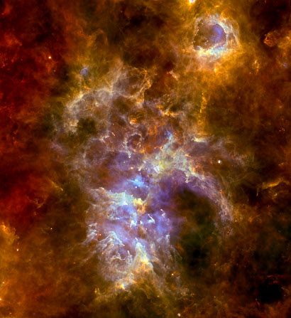

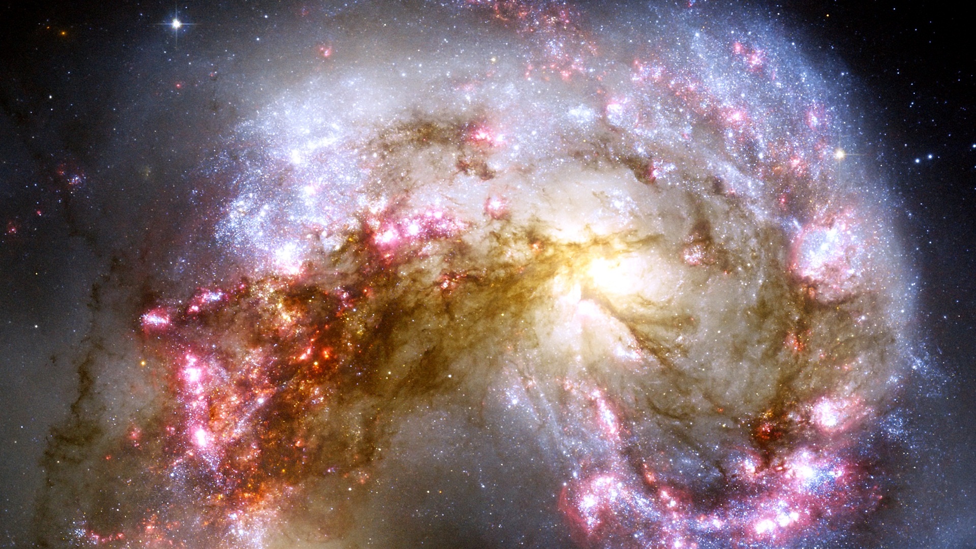 From left to right: The Orion nebular, the Carina star forming region,
the Tarantular nebular in the LMC and the cantral region of the
Antennae interacting galaxies.
From left to right: The Orion nebular, the Carina star forming region,
the Tarantular nebular in the LMC and the cantral region of the
Antennae interacting galaxies. Giant molecular clouds (GMCs) turn only a few to a few tens of per cent of their gas into stars, referred to as the Star Formation Efficiency (SFE - the ratio between mass converted into stars and total mass of the star forming region). Therefore, the potential of the embedded star cluster (star cluster which is still within its gas-cloud) is dominated by the remaining gas. The removal of this gas by feedback will leave the stars of the cluster in an out-of-equilibrium state. In most theoretical studies, the embedded star cluster is assumed to be in virial equilibrium and forms a spherically symmetric distribution of stars. In this case all studies agree that, to obtain a bound remnant star cluster, the SFE has to be extremely high - of order 30 per cent.
But, recent observations of embedded star forming regions show
that stars do form in spherically symmetric distributions, nor in
virial equilibrium. Instead they form in clumps and filaments, and
most likely dynamically cool.
 Data from Baumgardt and Kroupa 2007
credit: University of Exeter
Star formation in filamentary structures are studied by various groups using state-of-the-art SPH codes on very fast super-computers (see example to the left). These simulations are very time-consuming (many months/years of CPU-time) on the one hand and therefore cannot provide a statistical significant parameter search. On the other hand, these simulations lack the exact collisional stellar dynamical treatment of the newly formed stars. Furthermore, it is almost impossible to isolate the influence one particular parameter has on the outcome of the whole simulations.
Fast Idealised Models
In this project we try to assess the influence of each ingredient to the outcome separately by using very fast highly idealised models. For this we make use of the state-of-the-art direct N-body code N-body 6. This code provides us with the exact stellar dynamical treatment of the young stars and allows us to perform dozens or hundreds of simulations with the same parameter set to obtain statistical significant results. Finally, we can use the code in a way that we can introduce one or more parameter each time and separately. Therefore, our models are providing a completely complementary insight into the star cluster formation problem. Our initial conditions are a fractal distribution of stars (fractal dimension D=1.6; an example is shown below) embedded in a smooth analytical background representing the residual gas of the embedded cluster. All of our model start with an overall SFE = 0.2. In terms of the old simulations this means that none of our initial distributions should form a bound cluster. To mimic very fast and maximal destructive gas expulsion we remove the background potential instantaneously.
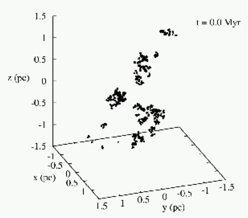 fractal initial conditions used in this project
The Erasure of Substructure
In a first experiment we asked how fast can we erase the substructure of our initial distribution of stars. We use small spherical clumps of stars instead of a fractal distribution and follow the dynamics counting how many clumps remain with time. The results are shown below. We see that substructure is erased very fast, i.e. exponentially, but maybe not fast enough.
 The erasure of substructure. We show the number of clumps
versus the time measured in initial crossing times of the system.
The erasure of substructure. We show the number of clumps
versus the time measured in initial crossing times of the system.
The Local Stellar Fraction (LSF)
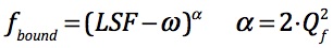
Instead of the overall SFE, which does not vary with time even though we have a highly dynamical system, we find that the LSF (local stellar fraction = an instantaneous SFE, measured at the varying half-mass radius at exactly the time of gas-expulsion) is a better description to predict the final bound mass fraction f_bound, i.e. how many stars of the embedded cluster remain bound to each other after gas-expulsion. This is particularly true as soon as the initial fractal distribution had enough time to settle into a virial equilibrium, i.e. when we have a late gas expulsion. We are able to quantify this relation as:

where f_bound is the fraction of stars bound after gas expulsion and ω = 0.14 is an off-set, determined through our simulations. Below this off-set we do not see any surviving cluster. We still see a lot of scatter in the results which may be due to a second parameter.
We dub the time of early gas-expulsion as the 'chaotic' regime, as our proposed parameter, the LSF no longer predicts the bound-mass fraction, Here we clearly see that the survival of our star cluster has to depend on a second parameter. We suspect that the virial ratio at time of gas expulsion plays an important role in our experiments.

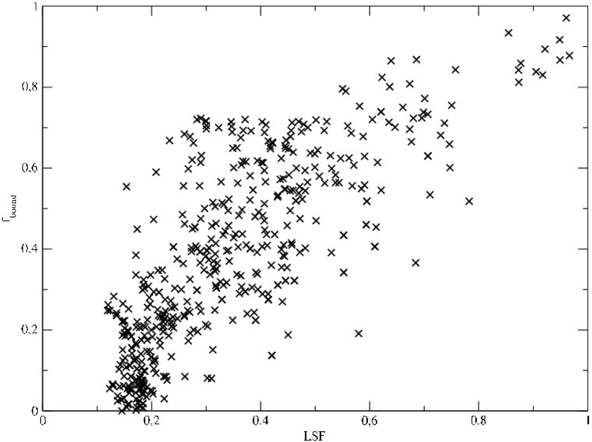 Bound fraction as function of the LSF for late gas expulsion. (left)
The 'chaotic' regime. (right)
Bound fraction as function of the LSF for late gas expulsion. (left)
The 'chaotic' regime. (right) A new time-scale
The young embedded star clusters are not in virial equilibrium, even though in most of our simulations the stars have virialised velocities inside the embedded cluster. But they are not forming a spherically symmetric distribution. What we see in our simulations is an initial collapse into the centre and an oscillation of the star distribution afterwards until we reach a final spherically symmetric and virialised distribution. Also the instantaneous virial state of our stellar distribution does oscillate.
Measuring time in initial crossing times of the system is not a correct measure of the dynamical state. We choose a new time-scale T_Q, which measures time in oscillations of the instantaneous virial parameter Q_f. With this new time-scale we can determine at which instant our distribution has exactly Q_f=0.5 and when do we see extremes in the virial parameters.
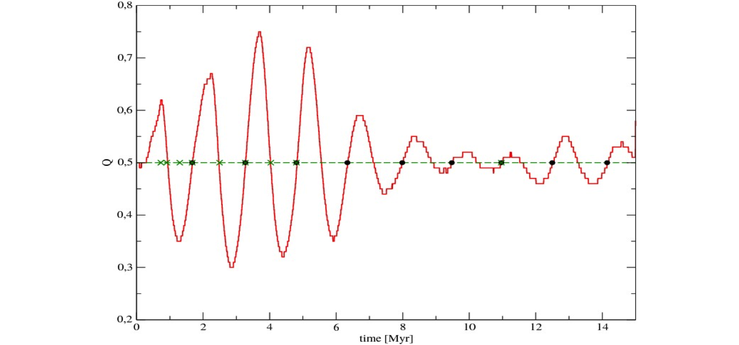 The Q oscillations of one of our simulations.
The importance of the virial ratio
We suspected that we have a second important parameter to take into account, namely the actual virial ratio of the stars at exactly the time of gas-expulsion, which we call Q_f, to distinguish with the virial ratio at which the embedded cluster is born (Q_i). We find that we can generalise Eq.1 in the following sense to again be able to predict the results of our simulations:
which reproduces Eq.1 within the error-bars. Still, for low LSF and Q_f values this relation raises very steeply so that with the remaining scatter, we still see in our results, the prediction of the final bound mass is impossible.

 The dependency of f_bound as function of LSF and Q_f. Left: the
fitted curves; Right: the theoretical curves.
The dependency of f_bound as function of LSF and Q_f. Left: the
fitted curves; Right: the theoretical curves.
A Quick Theoretical Insight
Please find a short description of the theory written in this PDF document. The fitting curves are shown above in the right panel.
Influence of the background
The remaining gas in our simplified simulations is modeled as a static background potential, which then is removed to mimic gas-expulsion. We investigated if the shape of this potential has any influence on the outcome of our results. We varied the potential from an uniform sphere to a highly concentrated Plummer distribution but our results showed that the answer of the star distribution (fractal distribution with fractal dimension 1.6) is almost completely independent to the shape of the gas potential. Simulations with the same initial conditions of the stars formed similar denser configurations before gas expulsion. This result was on one hand reassuring that our simplified models are quite insensitive to the choice of static potential and on the other hand allowed us to probe different regions of the LSF, as concentrated backgrounds have more remaining gas within the star distribution than e.g. an uniform sphere.
The influence of the IMF
As stars do not have the same mass, we included now in our models a standard Kroupa IMF (initial mass function) for stars between 0.1 and 120 M_sun. We see in our results, so far, that the internal evolution of the star distribution is faster. Especially, for dense systems, we find that the bound fractions measured are well below the trend we determined for equal mass particles.
This result shows that the internal processes, like scattering of stars of different masses, are at least equally if not more important for the destruction of young star clusters. I.e. the usual suspect called "gas-expulsion" may be innocent!
Mass-segregated Models
We perform models where the massive stars (M > 4 Msun) are randomly distributed, models in which we place all massive stars within the inner 0.5 pc of our fractal and models in which the massive stars are outside of the innermost pc.
With the initial contraction of our fractal we observe a mass-segregated star cluster, as soon as the first Q oscillation is over. I.e. with fractal initial conditions it is not important where massive stars are born, but as soon as the cluster looks more spherical, it is already mass-segregated.
While this result is reassuring, telling us that all star clusters are mass-segregated to begin with, it gives us no clue to where the massive stars are born.
Advanced SPH models
In the latest results we make use of the software package AMUSE. We run combined SPH and direct N-body models to simulate a live gas background (SPH) and the movements of the stars with high precision (direct N-body).
Evolution of Q and the LSF
First, we compare the amplitude of the Q oscillation measured by |Q-0.5|. How quickly this quantity drops to zero means how quickly the cluster can reach equilibrium and erase primordial substructure. We measure the mean value of |Q-0.5| for the 20 fractal clusters used in this work and show the results in the figure below where the blue lines are the means with blue shaded areas as the standard deviation. Black dashed lines represent the same quantities measured in the simulations with static background with the central line as the mean and the two other lines as the standard deviation.

We notice that there is no significant difference between the static and the live gas case. Neither with initially cold (bottom panel) or initially warm cluster a significant difference can be found. Still, in both panels the amplitude of the live gas case seems to remain slightly above the static potential case with standard deviation quite higher in the initially warm case. However, the difference is smaller than one sigma and could be explained by the difference in the numerical integrators used in the static and the live gas case.
With the same method we obtain the time averages of the LSF. The resulting LSF evolution is shown in the figure below. Simulations with a live gas background show a higher LSF than in the static case, but still within the one sigma deviation, so the difference is not significant. However, if we assume that the gas background remains as a Plummer sphere of Rpl = 1.0 pc, then the only possibility to raise the LSF is a decrease of the half mass radius of the stars. The main reason for the half mass radius to decrease is the interchange of angular momentum between the stars and the gas. The next figure shows the evolution of the angular momentum for the stars (dashed lines) and the gas (dotted lines). The top panel shows the mean angular momentum L relative to the total initial momentum Ltot,i for fractals with Qi = 0.5 shadows represent the standard deviation. The bottom panel shows fractals with Qi = 0.0. Since the clusters start with no initial velocities, hence no initial angular momentum, values are measured with respect to the final total angular momentum of the cluster Ltot,f.


For the initially warm case, we see that while the total angular momentum is more or less conserved, the gas obtains angular momentum from the stars, fast in the relaxation phase and slowly after the clusters rearrange causing a decrease in the velocities of the stars and thus a decrease in the half mass radius. As we can see from the standard deviation gas can gain up to 20% of the initial angular momentum in the warm case.
While in the initially cold case this interchange seems to be more important, this is only because the value of the initial angular momentum is lower. In this case stars start with no velocities and Ltot,i is zero so all the angular momentum that the cluster reaches comes from the violent initial relaxation and does not increase too much. In fact the maximum angular momentum for the gas is quite similar in both cases with 17.3 +/- 0.7 Msun pc km/s for the initially warm case and only a 20% lower in the cold case with 14.1 +/- 0.5 Msun pc km/s. Thus the interchange of momentum does not depend on the initial total angular momentum budget. No matter the initial conditions the gas will obtain more or less the same increase of angular momentum, most of it will come from the energy of the stars.
A big difference between simulations with live gas background and the static case comes from the interchange of energy between the stars and the gas. While in the static case stellar angular momentum is conserved, we have shown that the inclusion of a gas background is able to evolve results in a reduction of angular momentum of the same order no matter the initial conditions of the stars. This decrease of energy of the stars results in a decrease of the half mass radius of the stars. Since we have shown that the gaseous distribution remains quite stable especially with a low SFE, we conclude that the observed decrease in the half mass radius and therefore raise of the LSF originates only from the interchange of energy between the gaseous and stellar component.
Gas Expulsion In Highly Substructured Gas Distributions
We perform star formation simulations with the purpose of recreate the substructure of the gas and a consequent stellar distribution, thus we are not interested in the microscopic details of star formation which are very computationally expensive and would exhaust all our recurses into one single simulation. Instead we perform several cheaper star formation simulations to obtain sufficient results to obtain statistics. We know from our previous studies, that working with substructured distributions results could change from one random realization to another.
We setup of a turbulent molecular cloud of Mgas,i = 2500 Msun distributed in an initially uniform sphere of Rcl = 1.5 pc at a temperature of T = 10 K, that ends up in a Nstar = 1000 equal mass stellar distribution of Mstar = 500 Msun embedded in a filamentary cloud of gas of Mgas,f = 2000 Msun matching a SFE= 0.2. This filamentary cloud of gas and star distribution is used as initial condition to then either evolve the cloud for some time with sensitive constraints to avoid further collapse or remove the gas just after the 1000 star particles form. We only create equal mass particles since the inclusion of an IMF is a problem that is been studied independently (Dominguez et. al. in preparation)
With this setup the initial mean Jeans mass of the cloud is Mj ≈ 1 Msun which means that our cloud has ∼ 2500 Mj that is more than enough to form 1000 equal mass particles. We use 250K SPH particles to perform our simulation, according to Bate et al. (2003) the minimum SPH particles needed to resolve fragmentation correctly is 1.5Nsmooth per Jeans mass. The minimum Jeans mass that we are able to resolve with our setup is 0.75 Msun , however in our simulations we obtain densities above 109 Msun /pc3 with local Jeans masses of ∼ 0.0005 Msun . To properly resolve such densities in a cloud of the present size and mass, we would need 375 million SPH particles which is impossible to run with the computational resources at hand. However, in this work we are focused in the large scale substructure and we ignore this resolution problem for now since we are not interested in the local detail of fragmentation and star formation. In contrast, we are able to perform several cheap simulations instead of one single very expensive simulation.

A random velocity field is a mixture of two independent velocity fields: a compressive (curl-free) field, a and a solenoidal (divergence-free) field (Federrath et al., 2009). In a divergence-free field velocities are oriented in a way that the cloud does not expand or contract as a whole. In this case the contraction of the cloud is only caused by the self gravity of the cloud in overdense regions. On the other hand the curl-free velocity field avoids the net rotation of the cloud, giving priority to either compressive or expansive velocities. In terms of substructure, what we can see for example in the figure below and also in Figure 1 of Federrath et al. (2009) is that the curl-free part of a velocity field is mostly responsible for most of the filamentary structure in star forming regions, while in divergence-free fields star formation seems to happen in a more “uniform” way. Regardless these differences in the turbulent modes, there is no significant difference in the final stellar distribution in our star formation simulations.

The similarity of global parameters regardless the field type is in agreement with Girichidis et al. (2012) and Lomax et al. (2015) where the same turbulent modes have been tested on star formation on smaller clouds of less than 100 Msun in mass and less than 0.1 parsec in radius that form less than 500 low mass stars. The differences found are significant in the amount of high mass stars relative to low mass stars , and the kinds of fragmentation of the clouds (Lomax et al., 2015) however both cases are not relevant to this work since we force the formation of equal mass particles and our resolution is not enough to distinguish the different kind of fragmentation. In terms of substructure Girichidis et al. (2012) showed that in general curl-free modes of turbulence form slightly more substructured clusters than divergence-free modes, i.e., Ccomp Cmix Csol which agrees with our results. However, statistically, these differences are not significant in our simulations. Girichidis et al. (2012) conclude that these similarities between stellar distributions formed in different turbulent modes are because the newborn stars quickly decouple from its parent cloud dynamically, and N-body interactions dominate the motion of the stellar cluster. The continuous formation of stars with sub-virial velocities lead to a global sub-virial state which is in agreement with our simulations.
In comparison with to initial conditions stated above we now form clusters with 2.5 pc radius and a SFE of about 24%, slightly higher than the setup SFE of 20% since there is always some gas outside of Rmax. We obtain distributions with lower C parameters ,i.e. with the turbulent setup we obtain higher substructured clusters than the D = 1.6 stellar distributions used in the Plummer background case. However, the new distributions show a higher initial LSF, this is a consequence of the shape of the background gas that is not concentrated in the center like a Plummer sphere, instead it is generally concentrated in a filamentary structure around the center of mass of the cloud. Furthermore, the half mass radius in the turbulent setup is smaller which means that we obtain a more centrally concentrated cluster in comparison with the fractal method described by Cartwright and Whitworth (2004).
Velocity dispersions in the turbulent setup are almost identical to the ones in the warm Plummer background case with sigma_star about 1 km/s. Considering that the Qf = 0.3 for the stars in the turbulent cloud and the distributions are globally more extended than the Plummer background case, this already tells us something about the gravitational potential that the stars feel in a filamentary star formation scenario. Since the distributions are more extended, it is reasonable to think that the potential energy, felt by the stars, should decrease. However, the results show the opposite: the potential energy in a filamentary gas needs to be higher so sigma_star (and in consequence the kinetic energy) remains equal for a low value of Qf. This increase is because in the turbulent setup, even though gas and stars decouple, stars are quite near to the densest regions of the cloud, this would increase the potential energy of the stars decreasing the value of Qf.
Below we show several parameters for both AEOS and SGO sets of simulations. Different line types show the different velocity field type from which stars were born, with dashed lines for the curl-free field, dot dashed lines for the divergence-free field and mixed velocity field is shown as a solid line. The evolution of the spatial distributions for the gas and the stars are shown in the following two figures where each set of 6 panels show the evolution of the cluster under the two setups, self-gravity turned off (top panels) and the adiabatic EOS (bottom panels) at three points of the evolution: the beginning of the embedded phase (left panels), after 1 Myr (middle panels) and at 2 Myr of evolution (right panels). These points of the evolution also represent the points were we have expelled the gas that we will analyse in the next section.


We can see the difference in the evolution of the half mass radius in the first panel of the first figure where simulations with a curl-free velocity field born with a more extended stellar distribution than the other two field types. Later evolution depends of the treatment of the gas.
An adiabatic EOS for the gas causes the initially filamentary gas to rearrange in small clumps that eventually merge into bigger clumps as we can see in the bottom panels of last two figures these gaseous clumps are strong enough to attract nearby stellar clumps so stars and gas couple again merging into a bigger clump. Eventually we would obtain a similar situation than explained above, however 2 Myr is not enough to erase all the primordial substructure. How fast substructure is erased will depend of how extended the initial distribution is, this is confirmed by the C parameter (last panel of first figure) that show how clusters born in a curl-free velocity field (usually more extended) take more time to erase primordial substructure that is also higher for curl-free simulations.
In the case of SGO simulations, the gas is dispersed by the initial velocity of the gas and it is only attracted by the gravity of the stars. This is not enough to retain the fast gas particles. Rh stays higher than in the adiabatic case since the background potential is weaker. For the same reason the LSF raises to values above 60%. Substructure also remains higher, which we can see in the evolution of the C parameter. Even after 2 Myr of embedded evolution clusters without self-gravity for the gas never leave the “clumpy” regime (C less than 0.8).
The difference in the substructure of the stars and the concentration of the gas in both cases have critical consequences in the values of the structural parameters A and B (see full thesis for detailed explanation). The parameter A, which only depends on the stars, shows a strong decrease in the adiabatic case in contrast with the small decrease the simulations with no self-gravity for the gas. The parameter A increments with substructure which explains the high decrease in the adiabatic case (where substructure is erased efficiently) in comparison with the case without self-gravity. The evolution of the parameter B shows that in both cases the effective potential energy decreases. The parameter B is also proportional to substructure so it decreases with time as substructure is erased. However, we can see that the big change in the structure parameters originates mainly from the stellar component, i.e., the parameter A. This change causes that the B/A ratio split very clearly the two scenarios with low B/A ratios for simulations with no gaseous self-gravity and high values for the adiabatic simulations.
The rate at which substructure is erased also affects the dynamical state of the cluster. In the adiabatic case where substructure is erased quickly, the cluster reaches virial equilibrium faster than the case without self-gravity. When the background potential is weaker, the merging of clumps is supressed and the relative low velocities between each clump remain the same for a longer time. A merging results in several two body encounters that raise the kinetic energy (and hence the velocity dispersion), increasing the value of Q. In the SGO case this doesn’t happen and velocities remain similar during the 2 Myr that we have follow the evolution as we can see in the values of the velocity dispersion.
After following the evolution of the embedded star clusters with two extremes treatments for the background gas, we expel the gas instantaneously at 0, 1 and 2 Myr after 1000 stars have formed in the star formation phase. Then we measured the fraction of bound stars at 15 Myr after the moment of gas expulsion.
We can see in the figure below the results of the measurements of fbound together with the estimations from our models as errorbars and crosses for the two different treatments of the background gas. SGO simulations are shown in the left panels and AEOS simulations are shown in the right panels for the different moments of gas expulsion.

The high survival rates of the simulations expelling the gas at 0 Myr and SGO that are explained mainly by the low Qf and B/A ratios. Both parameters keep low in SGO simulations in contrast with the AEOS simulations where both parameters increase with time. In SGO simulations the LSF does not help to estimate fbound and bound fractions are mainly estimated by Qf . Considering substructure into the models does not always increment accuracy as we can see some crosses inside the errorbars in the figure above, however we will see later that in general it does a better job.
For AEOS simulations a similar trend to simulations with a Plummer Background potential araises. This is because in general this simulations tend to erase substructure, i.e., the ratio B/A increases to values near 1 and at the same time the embedded star cluster quickly reaches equilibrium (Q evolves to 0.5) in contrast with the SGO simulations were Q remains low for long times.
A closer look to the crosses and the errorbars in the figure shows that the model with substructure does, in general, a better job when substructure is high. However everything seems to be fairly well explained when measuring the effective Qf and considerations of substructure does not improve the predictions significantly. Hence, we have to quantify how well the models represent the results from all the simulations in this work.
The next figure shows the differences between the analytical models, i.e. our analytical predictions, with the different considerations and the measured bound fractions for all the simulations performed with a live gas background. We measure the standard deviation from the analytical model considering four cases: Models not considering substructure, i.e., assuming B/A = 1 (top panels); models con- sidering substructure through the numerical measurement of the structure parameters A and B (bottom panels): Models where the value of Qf is measured considering the mean velocity of the whole cluster, i.e., the global Qf (left panels); and models where Qf is measured by knowing the mean velocity of the clump that finally survives gas expulsion a priori, i.e., the effective Qf (right panels). We can see no changes when considering the global Qf or the effective Qf , i.e., shaded areas in the top panels are the same than in the bottom panels, this is because, in general, we obtain high bound fractions for all the simulations with a live gas background, with the exception of a small group of low LSF simulations that have not affected the results. Considering the structural parameters only improves our model on a 1% level as we can see by comparing the left panels with the right panels of the figure. But this is only true for simulations with fbound 0.3.

Including or not the structural parameters we can see that all the simulations performed utilizing a live gas background, even the simulations where gas expulsion happens at the beginning of the embedded phase when gas and stars are highly substructured, we can estimate the bound fractions with about 10% of uncertainly. This results shows that the inclusion of an arbitrary distribution for the gas and the stars does not result in an unpredictable scenario, in fact this results suggests that it is possible to predict how much mass a cluster can retain in any distribution if it is possible to measure at least the virial ratio and the LSF without caring for the presence of substructure. However, we must keep in mind that we test these models in equal mass stellar distributions. Inclusion of an initial mass function could alter the results depending of the level of mass segregation at the moment of gas expulsion since we don’t know how much it will affect the values of the structure parameters that we have shown are not very important but we haven’t reached extremes values yet that could be possible with massive stars. How much an IMF will affect the results is a question that we will explore in a future work.
This work is/was supported by the following grants:
- FONDECYT postdoctorado No.3120135; PI: Rory Smith, hosting professor: Michael Fellhauer
- FONDECYT regular No.1130521; PI: Michael Fellhauer
- BASAL: CATA - Centro de Astrofisica y Tecnologias Afines
- CONICYT beca para Magister; Juan-Pablo Farias Osses, supervisor: Michael Fellhauer
M. Fellhauer, R. Smith, S. Goodwin, R. Slater, M. Blana, J.P. Farias, R. Dominguez